Big O notation is a way of expressing the efficiency of an algorithm in terms of how its running time or space requirements grow as the input size increases. The Big O time complexity chart provides a visual representation of how different algorithms compare in terms of their efficiency.
For example, an algorithm with O(1) time complexity means that its running time is constant, regardless of the input size. On the other hand, an algorithm with O(n) time complexity means that its running time grows linearly with the input size.

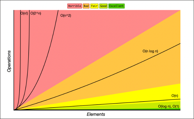
Common Time Complexities in the Chart
The Big O time complexity chart typically includes common time complexities such as O(1), O(log n), O(n), O(n log n), O(n^2), and O(2^n). Understanding these different time complexities can help developers choose the most efficient algorithm for a given problem.
For example, an algorithm with O(log n) time complexity is more efficient than an algorithm with O(n) time complexity for large input sizes, as the former grows logarithmically while the latter grows linearly.
Using the Big O Time Complexity Chart
When analyzing algorithms, it’s important to consider their time complexity and compare them using the Big O time complexity chart. By selecting algorithms with lower time complexities, developers can optimize their code and improve its performance.
Additionally, understanding the Big O time complexity chart can help developers anticipate how an algorithm will perform as the input size increases, allowing them to make informed decisions when designing and implementing algorithms.